[python]代码库
import torch
import torch.nn as nn
import matplotlib.pyplot as plt
import numpy as np
#import os
#os.environ["KMP_DUPLICATE_LIB_OK"] = "TRUE"
torch.manual_seed(10)
# ========生成数据=============
sample_nums = 100
mean_value = 1.7
bias = 1
n_data = torch.ones(sample_nums, 2)
x0 = torch.normal(mean_value * n_data, 1) + bias # 类别0数据
y0 = torch.zeros(sample_nums) # 类别0标签
x1 = torch.normal(-mean_value * n_data, 1) + bias # 类别1数据
y1 = torch.ones(sample_nums) # 类别1标签
train_x = torch.cat((x0, x1), 0)
train_y = torch.cat((y0, y1), 0)
# ==========选择模型===========
class LR(nn.Module):
def __init__(self):
super(LR, self).__init__()
self.features = nn.Linear(2, 1)
self.sigmoid = nn.Sigmoid()
def forward(self, x):
x = self.features(x)
x = self.sigmoid(x)
return x
lr_net = LR() # 实例化逻辑回归模型
# ==============选择损失函数===============
loss_fn = nn.BCELoss()
# ==============选择优化器=================
lr = 0.01
optimizer = torch.optim.SGD(lr_net.parameters(), lr=lr, momentum=0.9)
# ===============模型训练==================
for iteration in range(1000):
# 前向传播
y_pred = lr_net(train_x) # 模型的输出
# 计算loss
loss = loss_fn(y_pred.squeeze(), train_y)
# 反向传播
loss.backward()
# 更新参数
optimizer.step()
# 绘图
if iteration % 20 == 0:
mask = y_pred.ge(0.5).float().squeeze() # 以0.5分类
correct = (mask == train_y).sum() # 正确预测样本数
acc = correct.item() / train_y.size(0) # 分类准确率
plt.scatter(x0.data.numpy()[:, 0], x0.data.numpy()[:, 1], c='r', label='class0')
plt.scatter(x1.data.numpy()[:, 0], x1.data.numpy()[:, 1], c='b', label='class1')
w0, w1 = lr_net.features.weight[0]
w0, w1 = float(w0.item()), float(w1.item())
plot_b = float(lr_net.features.bias[0].item())
plot_x = np.arange(-6, 6, 0.1)
plot_y = (-w0 * plot_x - plot_b) / w1
plt.xlim(-5, 7)
plt.ylim(-7, 7)
plt.plot(plot_x, plot_y)
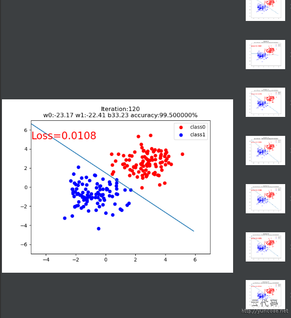
plt.text(-5, 5, 'Loss=%.4f' % loss.data.numpy(), fontdict={'size': 20, 'color': 'red'})
plt.title('Iteration:{}\nw0:{:.2f} w1:{:.2f} b{:.2f} accuracy:{:2%}'.format(iteration, w0, w1, plot_b, acc))
plt.legend()
plt.show()
plt.pause(0.5)
if acc > 0.99:
break
[代码运行效果截图]